Setting the Scene
Overview
Teaching: 10 min
Exercises: 0 minQuestions
What are we teaching in this course?
What motivated the selection of topics covered in the course?
Objectives
Setting the scene and expectations
Making sure everyone has all the necessary software installed
Introduction
The course is organised into the following sections:
Section 1: Software project example
Section 2: Unit testing
Before We Start
A few notes before we start.
Prerequisite Knowledge
This is an intermediate-level software development course intended for people who have already been developing code in Python (or other languages) and applying it to their own problems after gaining basic software development skills. So, it is expected for you to have some prerequisite knowledge on the topics covered, as outlined at the beginning of the lesson. Check out this quiz to help you test your prior knowledge and determine if this course is for you.
Setup, Common Issues & Fixes
Have you setup and installed all the tools and accounts required for this course? Check the list of common issues, fixes & tips if you experience any problems running any of the tools you installed - your issue may be solved there.
Compulsory and Optional Exercises
Exercises are a crucial part of this course and the narrative. They are used to reinforce the points taught and give you an opportunity to practice things on your own. Please do not be tempted to skip exercises as that will get your local software project out of sync with the course and break the narrative. Exercises that are clearly marked as “optional” can be skipped without breaking things but we advise you to go through them too, if time allows. All exercises contain solutions but, wherever possible, try and work out a solution on your own.
Outdated Screenshots
Throughout this lesson we will make use and show content from various interfaces, e.g. websites, PC-installed software, command line, etc. These are evolving tools and platforms, always adding new features and new visual elements. Screenshots in the lesson may then become out-of-sync, refer to or show content that no longer exists or is different to what you see on your machine. If during the lesson you find screenshots that no longer match what you see or have a big discrepancy with what you see, please open an issue describing what you see and how it differs from the lesson content. Feel free to add as many screenshots as necessary to clarify the issue.
Let Us Know About the Issues
The original materials were adapted specifically for this workshop. They weren’t used before, and it is possible that they contain typos, code errors, or underexplained or unclear moments. Please, let us know about these issues. It will help us to improve the materials and make the next workshop better.
$ cd ~/InterPython_Workshop_Example/data
$ ls -l
total 24008
-rw-rw-r-- 1 alex alex 23686283 Jan 10 20:29 kepler_RRLyr.csv
-rw-rw-r-- 1 alex alex   895553 Jan 10 20:29 lsst_RRLyr.pkl
-rw-rw-r-- 1 alex alex   895553 Jan 10 20:29 lsst_RRLyr_protocol_4.pkl
...
Exercise
Exercise task
Solution
Exercise solution
 code example
 ...
Key Points
Keypoint 1
Keypoint 2
Section 1: HPC basics
Overview
Teaching: 5 min
Exercises: 0 minQuestions
Question 1
Objectives
Objective 1
Section overview, what it’s about, tools we’ll use, info we’ll learn.
- Intro into HPC calculations and how they differ from usual ones
- Introducing code examples (CPU and GPU ones)
- A recap of terminal commands useful for remote work and HPC (+practical session: terminal commands)
- Different types of HPC facilities, how to choose one, LSST HPC infrastructure
Key Points
Keypoint 1
HPC Intro
Overview
Teaching: 5 min
Exercises: 0 minQuestions
Question 1
Objectives
Objective 1
- Intro into HPC calculations and how they differ from usual ones
Intro
Paragraph 1
Key Points
Keypoint 1
Intro code examples
Overview
Teaching: 30 min
Exercises: 20 minQuestions
What is the difference between serial and parallel code?
How do CPU and GPU programs differ?
What tools and programming models are used for HPC development?
Objectives
Understand the structure of CPU and GPU code examples.
Identify differences between serial, multi-threaded, and GPU-accelerated code.
Recognize common programming models like OpenMP, MPI, and CUDA.
Appreciate performance trade-offs and profiling basics.
Motivation for HPC Coding
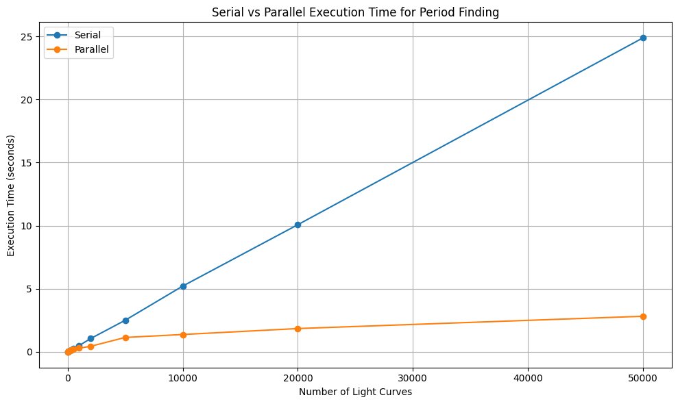
Most users begin with simple serial code, which runs sequentially on one processor. However, for problems involving large data sets, high resolution simulations, or time-critical tasks, serial execution quickly becomes inefficient.
Parallel programming allows us to split work across multiple CPUs or even GPUs. High-Performance Computing (HPC) relies on this concept to solve problems faster. We can visualise this by looking at an example of finding the period for light curves. The visualisation of this example is given below:
Serial Code Example (CPU)
Introduction to NumPy
Before diving into parallel computing or GPU acceleration, it’s important to understand how performance can already be improved significantly on a CPU using efficient libraries.
- One of the most widely used tools for this in Python is
NumPy. NumPy provides a fast and memory-efficient way to handle large numerical datasets using multi-dimensional arrays and vectorized operations. - While regular Python lists are flexible, they are not optimized for heavy numerical tasks. Looping through data element by element can quickly become a bottleneck as the problem size grows.
- NumPy solves this problem by providing a powerful N-dimensional array object and tools for performing operations on these arrays efficiently.
- Under the hood, NumPy uses optimized C code, so operations are much faster than using standard Python loops.
- NumPy also supports vectorized operations, which means you can apply functions to entire arrays without writing explicit loops. This not only improves performance but also leads to cleaner and more readable code.
- Using NumPy on the CPU is often the first step toward writing efficient scientific code.
- It’s a strong foundation before we move on to parallel computing or GPU acceleration. Now, we’ll see an example of how a simple numerical operation is implemented using NumPy on a single CPU core.
Example: Summing the elements of a large array using Serial Computation
import numpy as np
import time

array = np.random.rand(10**7)
start = time.time()
total = np.sum(array)
end = time.time()
print(f"Sum: {total}, Time taken: {end - start:.4f} seconds")
Exercise:
Modify the above to use a manual loop with
forinstead ofnp.sum, and compare the performance.
Solution
Replace
np.sum(array)with a manual loop usingfor.
Note: This will be much slower due to Python’s loop overhead.import numpy as np import time array = np.random.rand(10**7) start = time.time() total = 0.0 for value in array: total += value end = time.time() print(f"Sum: {total}, Time taken: {end - start:.4f} seconds")This gives you a baseline for how optimized
np.sumis compared to native Python loops.
Reference:
Parallel CPU Programming
Introduction to OpenMP and MPI
Parallel programming on CPUs is primarily achieved through two widely-used models:
OpenMP (Open Multi-Processing)
OpenMP is used for shared-memory parallelism. It enables multi-threading where each thread has access to the same memory space. It is ideal for multicore processors on a single node.
OpenMP was first introduced in October 1997 as a collaborative effort between hardware vendors, software developers, and academia. The goal was to standardize a simple, portable API for shared-memory parallel programming in C, C++, and Fortran. Over time, OpenMP has evolved to support nested parallelism, Single Instruction Multiple Data (vectorization), and offloading to GPUs, while remaining easy to integrate into existing code through compiler directives.
OpenMP is now maintained by the OpenMP Architecture Review Board, which includes organizations like Arm, AMD, IBM, Intel, Cray, HP, Fujitsu, Nvidia, NEC, Red Hat, Texas Instruments, and Oracle Corporation. OpenMP allows you to parallelize loops in C/C++ or Fortran using compiler directives.
Terminology
Nested Parallelism
- Nested parallelism occurs when a parallel task itself spawns additional parallel tasks. For example, imagine a program where each thread is responsible for a different data block, and within each block, more threads are launched to handle sub-tasks. This is useful when dealing with hierarchical or recursive algorithms but must be managed carefully to avoid performance penalties due to thread overhead.
Single Instruction, Multiple Data (SIMD) – Vectorization
- SIMD is a form of data-level parallelism where the same instruction operates on multiple data elements simultaneously. For instance, instead of adding two numbers at a time, SIMD allows processors to add pairs of numbers in parallel using wide registers (like 128-bit or 256-bit). Vectorized operations using NumPy or compiler intrinsics take advantage of this under the hood to speed up loops.
Offloading to GPUs
- Offloading refers to transferring compute-intensive tasks from the CPU to the GPU, which is optimized for parallel processing. This is particularly effective for operations that can be executed simultaneously on thousands of threads, like matrix multiplications in deep learning or simulations in scientific computing. Tools like CUDA, OpenCL, or libraries like CuPy and PyTorch help achieve this in Python.
Example: Running a loop in parallel using OpenMP
#include <omp.h>
#pragma omp parallel for
for (int i = 0; i < N; i++) {
    a[i] = b[i] + c[i];
}
Since C programming is not a prerequisite for this workshop, let’s break down the parallel loop code in detail.
Requirements:
- Add
#include <omp.h>to your code - Compile with
-fopenmpflag
Before we look at the explanation of the C code, we will first look at the Python Equivalent of this code
Python Equivalent of the Code Logic
def add_arrays(b, c):
     """
     Takes two lists `b` and `c`, adds corresponding elements,
     and returns the resulting list `a` where a[i] = b[i] + c[i].
     """
    # Make sure both lists are the same length
    assert len(b) == len(c), "Input arrays must be the same length"

    # Create an output list of the same size
    a = [0.0 for _ in range(len(b))]

    # Loop through and compute a[i] = b[i] + c[i]
    for i in range(len(b)):
        a[i] = b[i] + c[i]

    return a

 # Example usage
 N = 100000
 b = [i * 0.1 for i in range(N)]
 c = [i * 0.2 for i in range(N)]

 a = add_arrays(b, c)

 # Print first few values to verify
 print(a[:10])
Explanation of the C code
#include <omp.h>: Includes the OpenMP API header needed for all OpenMP functions and directives.#pragma omp parallel for: A compiler directive that tells the compiler to parallelize theforloop that follows.- The
forloop itself performs element-wise addition of two arrays (bandc), storing the result in arraya.How OpenMP Executes This
- OpenMP detects available CPU cores (e.g., 4 or 8).
- It splits the loop into chunks — one for each thread.
- Each core runs its chunk simultaneously (in parallel).
- The threads synchronize automatically once all work is done.
Output
- The output is stored in array
a, which will contain the sum of corresponding elements from arraysbandc. The execution is faster than running the loop sequentially.Real-World Analogy
Suppose you need to send 100 emails:
- Without OpenMP: One person sends all 100 emails one by one.
- With OpenMP: 4 people each send 25 emails at the same time — finishing in a quarter of the time.
Exercise: Parallelization Challenge
Consider this loop:
for (int i = 1; i < N; i++) {
  a[i] = a[i-1] + b[i];
}
Can this be parallelized with OpenMP? Why or why not?
Solution
No, this cannot be safely parallelized because each iteration depends on the result of the previous iteration (
a[i-1]).OpenMP requires loop iterations to be independent for parallel execution. Here, since each
a[i]relies ona[i-1], the loop has a sequential dependency, also known as a loop-carried dependency.This prevents naive parallelization with OpenMP’s
#pragma omp parallel for.However, this type of problem can be parallelized using more advanced techniques like a parallel prefix sum (scan) algorithm, which restructures the computation to allow parallel execution in logarithmic steps instead of linear.
MPI (Message Passing Interface)
MPI is used for distributed-memory parallelism. Processes run on separate memory spaces (often on different nodes) and communicate via message passing. It is suitable for large-scale HPC clusters.
MPI emerged earlier, in the early 1990s, as the need for a standardized message-passing interface became clear in the growing field of distributed-memory computing. Before MPI, various parallel systems used their own vendor-specific libraries, making code difficult to port across machines.
In June 1994, the first official MPI standard (MPI-1) was published by the MPI Forum, a collective of academic institutions, government labs, and industry partners. Since then, MPI has become the de facto standard for scalable parallel computing across multiple nodes, and it continues to evolve with versions like MPI-2, MPI-3, MPI-4, and finally MPI-5 released on June 5 2025 which add support for features like parallel I/O and dynamic process management.
Example: Implementation of MPI using the mpi4py library in python
from mpi4py import MPI

comm = MPI.COMM_WORLD
rank = comm.Get_rank()
size = comm.Get_size()

data = rank ** 2
all_data = comm.gather(data, root=0)
if rank == 0:
    print(all_data)
Explanation of the code
This example demonstrates a basic use of
mpi4pyto perform a gather operation using theMPI.COMM_WORLDcommunicator.Each process:
- Determines its rank (an integer from 0 to N-1, where N is the number of processes).
- Computes
rank ** 2(the square of its rank).- Uses
comm.gather()to send the result to the root process (rank 0).Only the root process gathers the data and prints the complete list.
Example Output (4 processes):
- Rank 0 computes
0² = 0- Rank 1 computes
1² = 1- Rank 2 computes
2² = 4- Rank 3 computes
3² = 9The root process (rank 0) gathers all results and prints:
[0, 1, 4, 9]
- Other ranks do not print anything.
This example illustrates point-to-root communication which is useful when one process needs to collect and process results from all workers.
Slurm Script to execute the code
#!/bin/bash
#SBATCH --job-name=mpi_hpc_ws
#SBATCH --output=mpi_%j.out
#SBATCH --error=mpi_%j.err
#SBATCH --partition=defaultq
#SBATCH --nodes=2
#SBATCH --ntasks=4
#SBATCH --time=00:10:00
#SBATCH --mem=16G

# Load required modules
module purge # Remove the list of pre loaded modules
module load Python/3.9.1
module list # List the modules

# Create a python virtual environment
python3 -m venv name_of_your_venv

# Activate your Python environment
source name_of_your_venv/bin/activate

# Run the MPI job
mpirun -np 4 python mpi_hpc_ws.py
Make sure your virtual environment has mpi4py installed and that your system has access to the OpenMPI runtime via mpirun. Adjust the number of nodes and tasks depending on the cluster policies.
Exercise:
Modify serial array summation using OpenMP (C) or
multiprocessing(Python).
References:
GPU Programming Concepts
GPUs, or Graphics Processing Units, are composed of thousands of lightweight processing cores that are optimized for handling multiple operations simultaneously. This parallel architecture makes them particularly effective for data-parallel problems, where the same operation is performed independently across large datasets such as matrix multiplications, vector operations, or image processing tasks.
Originally designed to accelerate the rendering of complex graphics and visual effects in computer games, GPUs are inherently well-suited for high-throughput computations involving large tensors and multidimensional arrays. Their architecture enables them to perform numerous arithmetic operations in parallel, which has made them increasingly valuable in scientific computing, deep learning, and simulations.
Even without explicit parallel programming, many modern libraries and frameworks (such as TensorFlow, PyTorch, and CuPy) can automatically leverage GPU acceleration to significantly improve performance. However, to fully exploit the computational power of GPUs, especially in high-performance computing (HPC) environments, explicit parallelization is often employed.
Introduction to CUDA
In HPC systems, CUDA (Compute Unified Device Architecture), a parallel computing platform and programming model developed by NVIDIA is the most widely used platform for GPU programming. CUDA allows developers to write highly parallel code that runs directly on the GPU, providing fine-grained control over memory usage, thread management, and performance optimization. It allows developers to harness the power of NVIDIA GPUs for general-purpose computing, known as GPGPU (General-Purpose computing on Graphics Processing Units).
A Brief History
- Introduced by NVIDIA in 2006, CUDA was the first platform to provide direct access to the GPU’s virtual instruction set and parallel computational elements.
- Before CUDA, GPUs were primarily used for rendering graphics, and general-purpose computations required indirect use through graphics APIs like OpenGL or DirectX.
- CUDA revolutionized scientific computing, deep learning, and high-performance computing (HPC) by enabling massive parallelism and accelerating workloads previously limited to CPUs.
How CUDA Works
CUDA allows developers to write C, C++, Fortran, and Python code that runs on the GPU.
- A CUDA program typically runs on both the CPU (host) and the GPU (device).
- Computational tasks (kernels) are written to execute in parallel across thousands of lightweight CUDA threads.
- These threads are organized hierarchically into:
- Grids of Blocks
- Blocks of Threads
- This can be visualised in the following form
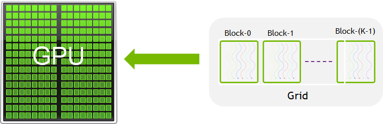
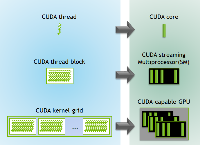
Figure Source:
Key Features
- Massive parallelism with thousands of concurrent threads
- Unified memory architecture for seamless CPU-GPU data access
- Built-in libraries for BLAS, FFT, random number generation, and more (e.g., cuBLAS, cuFFT, cuRAND)
- Tooling support including profilers, debuggers, and performance analyzers (e.g., Nsight, CUDA-GDB)
A CUDA program includes:
- Host code: Runs on the CPU, manages memory, and launches kernels.
- Device code (kernel): Runs on the GPU.
- Memory management: Host/device memory allocations and transfers.
To execute any CUDA program, there are three main steps:
- Copy the input data from host memory to device memory, also known as host-to-device transfer.
- Load the GPU program and execute, caching data on-chip for performance.
- Copy the results from device memory to host memory, also called device-to-host transfer.
Checking CUDA availability before running code
import cuda

if cuda.is_available():
    print("CUDA is available!")
    print(f"Detected GPU: {cuda.get_current_device().name}")
else:
    print("CUDA is NOT available.")
High-Level Libraries for Portability
High-level libraries allow easier GPU programming in Python:
- Numba: JIT compiler for Python; supports GPU via
@cuda.jit - CuPy: NumPy-like API for NVIDIA GPUs
- Dask: Parallel computing with familiar APIs
Example: Add vectors utlising CUDA using the numba python library
from numba_cuda import cuda
import numpy as np
import time

@cuda.jit
def add_vectors(a, b, c):
    i = cuda.grid(1)
    if i < a.size:
        c[i] = a[i] + b[i]

# Setup input arrays
N = 1_000_000
a = np.arange(N, dtype=np.float32)
b = np.arange(N, dtype=np.float32)
c = np.zeros_like(a)

# Copy arrays to device
d_a = cuda.to_device(a)
d_b = cuda.to_device(b)
d_c = cuda.device_array_like(a)

# Configure the kernel
threads_per_block = 256
blocks_per_grid = (N + threads_per_block - 1) // threads_per_block

# Launch the kernel
start = time.time()
add_vectors[blocks_per_grid, threads_per_block](d_a, d_b, d_c)
cuda.synchronize()  # Wait for GPU to finish
gpu_time = time.time() - start

# Copy result back to host
d_c.copy_to_host(out=c)

# Verify results
print("First 5 results:", c[:5])
print("Time taken on GPU:", gpu_time, "seconds")
Slurm Script to execute the code
The following script can be used to submit a GPU-accelerated Python job (numba_cuda_test.py) using Slurm:
#!/bin/bash
#SBATCH --job-name=Numba_Cuda
#SBATCH --output=Numba_Cuda_%j.out
#SBATCH --error=Numba_Cuda_%j.err
#SBATCH --partition=gpu
#SBATCH --nodes=1
#SBATCH --ntasks-per-node=1
#SBATCH --cpus-per-task=4
#SBATCH --mem=16G
#SBATCH --gpus-per-node=1
#SBATCH --time=00:10:00

# --------- Load Environment ---------
module load Python/3.9.1
module load cuda/11.2
module list

# --------- Check whether the GPU is available ---------
from numba import cuda
print("CUDA Available:", cuda.is_available())
# Activate virtual environment
source 'name_of_venv'/bin/activate # Here name_of_venv refers to the name of your virtual environment without the quotes

# --------- Run the Python Script ---------
 python numba_cuda_test.py
Make sure your virtual environment includes the numba-cuda python library to access the GPU.
Exercise:
Write a Numba or CuPy version of vector addition and compare speed with NumPy.
References:
CPU vs GPU Architecture
- CPUs: Few powerful cores, better for sequential tasks.
- GPUs: Many lightweight cores, ideal for parallel workloads.
Comparing CPU and GPU Approaches
| Feature | CPU (OpenMP/MPI) | GPU (CUDA) |
|---|---|---|
| Cores | Few (2–64) | Thousands (1024–10000+) |
| Memory | Shared / distributed | Device-local (needs transfer) |
| Programming | Easier to debug | Requires more setup |
| Performance | Good for logic-heavy tasks | Excellent for large, data-parallel problems |
Exercise:
Show which parts of the code execute on GPU vs CPU (host vs device). Read about concepts like memory copy and kernel launch from the CUDA C++ Programming Guide Chapter 5.
Reference: NVIDIA CUDA Samples
Summary
- Serial code is simple but doesn’t scale well.
- Use OpenMP and MPI for parallelism on CPUs.
- Use CUDA (or high-level wrappers like Numba/CuPy) for GPU programming.
- Always profile your code to understand performance.
- Choose your tool based on problem size, complexity, and hardware.
Key Points
Serial code is limited to a single thread of execution, while parallel code uses multiple cores or nodes.
OpenMP and MPI are popular for parallel CPU programming; CUDA is used for GPU programming.
High-level libraries like Numba and CuPy make GPU acceleration accessible from Python.
Command line for HPC and other remote facilities
Overview
Teaching: 5 min
Exercises: 0 minQuestions
Question 1
Objectives
Objective 1
- A recap of terminal commands useful for remote work and HPC (+practical session: terminal commands)
Intro
Paragraph 1
Exercise
Exercise task
Solution
Exercise solution
 code example
 ...
Key Points
Keypoint 1
HPC facilities
Overview
Teaching: 5 min
Exercises: 0 minQuestions
Question 1
Objectives
Objective 1
What are the IDACs
- IDACs idea: computational facilities from all over the world contribute their CPU hours and storage space
- Different types of IDACs: full DR storage, light IDACs, computation-only…
IDACs roster
A table with IDAC website, CPUs/GPU/Storage space data, Status (operational, construction, planned…), LSST and other surveys data stored, access info (command line/GUI), access policy (automated upon registration, personal contact needed, restricted to certain countries, etc), additional information (e.g. no Jupyter or best suited for LSST epoch image analysis).
Key Points
Keypoint 1
Section 2: HPC Bura
Overview
Teaching: 5 min
Exercises: 0 minQuestions
Question 1
Objectives
Objective 1
Section overview, what it’s about, tools we’ll use, info we’ll learn.
- HPC Bura, how to access it. Different authorization schemes used by the astronomical HPC facilities (+practical session: logging in to the Bura)
- Intro for computing nodes and resources
- Slurm as a workload manager (+practical session: how to use Slurm)
- Resource optimization (+practical session: running CPU and GPU code examples)
Key Points
Keypoint 1
Bura access
Overview
Teaching: 5 min
Exercises: 0 minQuestions
Question 1
Objectives
Objective 1
- HPC Bura, how to access it. Different authorization schemes used by the astronomical HPC facilities (+practical session: logging in to the Bura)
Intro
Paragraph 1
Exercise
Exercise task
Solution
Exercise solution
 code example
 ...
Key Points
Keypoint 1
Intro for computing nodes and resources
Overview
Teaching: 5 min
Exercises: 0 minQuestions
Question 1
Objectives
Objective 1
- Intro for computing nodes and resources
Intro
Paragraph 1
Key Points
Keypoint 1
Slurm
Overview
Teaching: 5 min
Exercises: 0 minQuestions
Question 1
Objectives
Objective 1
- Slurm as a workload manager (+practical session: how to use Slurm)
Intro
Paragraph 1
Key Points
Keypoint 1
Resource optimization
Overview
Teaching: 30 min
Exercises: 10 minQuestions
What is the difference between requesting for CPU and GPU resources using Slurm?
How can I optimize my slurm script to use the best resources for my specific task?
Objectives
Understand different types of computational workloads and their resource requirements
Write optimized Slurm job scripts for sequential, parallel, and GPU workloads
Monitor and analyze resource utilization
Apply best practices for efficient resource allocation
Understanding Resource Requirements
Different computational tasks have varying resource requirements. Understanding these patterns is crucial for efficient HPC usage.
Types of Workloads
CPU-bound workloads: Tasks that primarily use computational power
- Mathematical calculations, simulations, data processing
- Benefit from more CPU cores and higher clock speeds
Memory-bound workloads: Tasks limited by memory access speed
- Large dataset processing, in-memory databases
- Require sufficient RAM and fast memory access
I/O-bound workloads: Tasks limited by disk or network operations
- File processing, database queries, data transfer
- Benefit from fast storage and network connections
GPU-accelerated workloads: Tasks that can utilize parallel processing
- Machine learning, scientific simulations, image processing
- Require appropriate GPU resources and memory
Types of Jobs and Resources
When you run work on an HPC cluster, your job’s type determines how it will be scheduled and what resources it will use. Broadly, jobs fall into three categories:
-
Serial jobs
These use a single CPU core (or sometimes a single thread) to run all calculations. They don’t require communication between multiple processes. They’re ideal for workloads like simple data analysis, single-threaded simulations, or testing code. -
Parallel jobs
These use multiple CPU cores — sometimes across multiple nodes — to run tasks simultaneously. Parallel jobs often use MPI (Message Passing Interface) or OpenMP explained in the previous section to coordinate work. They’re suited for large-scale simulations or computations that can be split into many parts running at once. -
GPU jobs
These use Graphics Processing Units to accelerate certain types of workloads, especially those involving heavy numerical computation like deep learning, image processing, or large matrix operations. GPU jobs often also use CPU cores for parts of the workflow.
Once you know your job type, you can select the correct SLURM partition (queue) and request the right resources:
| Job Type | SLURM Partition | Key SLURM Options | Example Use Case |
|---|---|---|---|
| Serial | serial |
--partition, no MPI |
Single-thread tensor calc |
| Parallel | defaultq |
-N, -n, mpirun |
MPI simulation |
| GPU | gpu |
--gpus, --cpus-per-task |
Deep learning training |
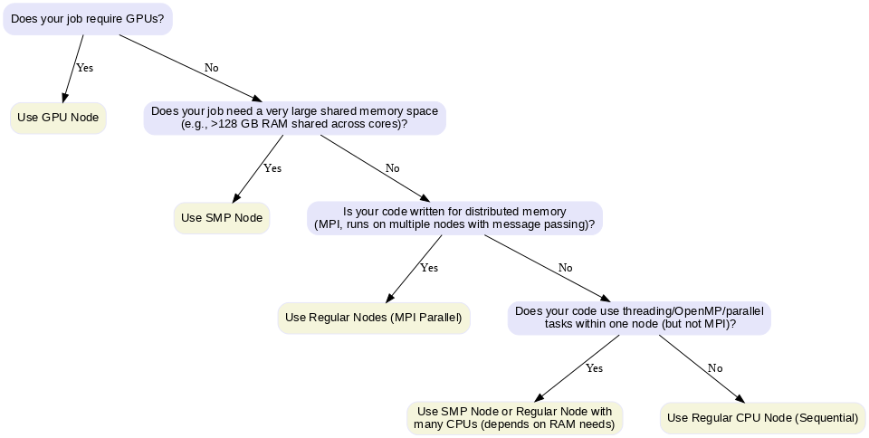
Choosing the Right Node
- Regular Node: For MPI-based distributed jobs or simple CPU tasks.
- SMP Node (Symmetric Multiprocessing): For jobs needing large shared memory (big matrices, in-memory data) or multi-threaded code (OpenMP, R, Python multiprocessing).
- In an SMP system, multiple CPUs (cores) share the same physical memory and can access it at the same speed. This architecture is ideal when tasks need frequent access to a common memory space without the communication overhead of distributed systems.
- GPU Node: For massively parallel computations on GPUs (e.g., CUDA, TensorFlow, PyTorch).
Decision chart for Choosing Nodes:
Example
For understanding how we can utilise different resources available on the HPC for the same computational task, we take the example of a python code which calculates the Gravitational Deflection Angle defined in the following way:
Deflection Angle Formula
For light passing near a massive object, the deflection angle (α) in the weak-field approximation is given by:
α = 4GM / (c²b)
Where:
- G = Gravitational constant (6.67430 × 10⁻¹¹ m³ kg⁻¹ s⁻²)
- M = Mass of the lensing object (in kilograms)
- c = Speed of light (299792458 m/s)
- b = Impact parameter (the closest approach distance of the light ray to the mass, in meters)
Computational Task Description
Compute the deflection angle over a grid of:
- Mass values: From 1 to 1000 solar masses (10³⁰ to 10³³ kg)
- Impact parameters: From 10⁹ to 10¹² meters
Generate a 2D array where each entry corresponds to the deflection angle for a specific pair of mass and impact parameter. Now we will look at how we will implement this for the different resources available on the HPC.
Sequential Job Optimization
Sequential jobs run on a single CPU core and are suitable for tasks that cannot be parallelized.
In an HPC environment, you might encounter sequential jobs when:
- Running legacy scientific codes that were never written for parallel execution.
- Doing data preprocessing or postprocessing steps that are inherently single-threaded.
- Running debugging or testing on a small portion of your code before scaling up to parallel execution.
- Executing small utilities like file format conversion, simple simulations, or statistical analyses that finish quickly and don’t need multiple cores.
Although these jobs only use one core, they can still benefit from HPC resources such as faster CPUs, high memory availability, and optimized software libraries.
Sequential Job Script Explained
#!/bin/bash
#SBATCH -J jobname                    # Job name for identification
#SBATCH -o outfile.%J                 # Standard output file (%J = job ID)
#SBATCH -e errorfile.%J               # Standard error file (%J = job ID)
#SBATCH --partition=serial            # Use serial queue for single-core jobs
./[programme executable name]          # Execute your program
Script breakdown:
#!/bin/bash: Specifies bash shell for script execution#SBATCH -J jobname: Sets a descriptive job name for easy identification in queue#SBATCH -o outfile.%J: Redirects standard output to a file with job ID#SBATCH -e errorfile.%J: Redirects error messages to separate file#SBATCH --partition=serial: Specifies the queue/partition for sequential jobs
Example: Gravitational Deflection Angle Sequential CPU
import numpy as np
import time
import matplotlib.pyplot as plt
import os
import matplotlib.colors as colors

# Constants
G = 6.67430e-11
c = 299792458
M_sun = 1.98847e30

# Parameter grid
mass_grid = np.linspace(1, 1000, 10000)  # Solar masses
impact_grid = np.linspace(1e9, 1e12, 10000)  # meters

result = np.zeros((len(mass_grid), len(impact_grid)))

# Timing
start = time.time()

# Sequential computation
for i, M in enumerate(mass_grid):
    for j, b in enumerate(impact_grid):
        result[i, j] = (4 * G * M * M_sun) / (c**2 * b)

end = time.time()

print(f"CPU Sequential time: {end - start:.3f} seconds")

result = np.save("result_cpu.npy", result)
mass_grid = np.save("mass_grid_cpu.npy", mass_grid)
impact_grid = np.save("impact_grid_cpu.npy", impact_grid)

# Load data
result = np.load("result_cpu.npy")
mass_grid = np.load("mass_grid_cpu.npy")
impact_grid = np.load("impact_grid_cpu.npy")

# Create meshgrid
M, B = np.meshgrid(mass_grid / 1.989e30, impact_grid / 1e9, indexing='ij')

# Create output directory
os.makedirs("plots", exist_ok=True)

plt.figure(figsize=(8,6))
pcm = plt.pcolormesh(B, M, result,
                      norm=colors.LogNorm(vmin=result[result > 0].min(), vmax=result.max()),
                      shading='auto', cmap='plasma')

plt.colorbar(pcm, label='Deflection Angle (radians, log scale)')
plt.xlabel('Impact Parameter (Gm)')
plt.ylabel('Mass (Solar Masses)')
plt.title('Gravitational Deflection Angle - CPU')

plt.tight_layout()
plt.savefig("plots/deflection_angle_cpu.png", dpi=300)
plt.close()

print("CPU plot saved in 'plots/deflection_angle_cpu.png'")
Sequential Job Script for the Example
#!/bin/bash
#SBATCH --job-name=HPC_WS_SCPU # Provide a name for the job
#SBATCH --output=HPC_WS_SCPU_%j.out # Request the output file along with the job number
#SBATCH --error=HPC_WS_SCPU_%j.err # Request the error file along with the job number
#SBATCH --partition=serial
#SBATCH --nodes=1 # Request one CPU node
#SBATCH --ntasks=1 # Request 1 core from the CPU node
#SBATCH --time=-01:00:00 # Set time limit for the job
#SBATCH --mem=16G #Request 16GB memory

# Load required modules
module purge # Remove the list of pre loaded modules
module load Python/3.9.1
module list

# Create a python virtual environment
python3 -m venv name_of_your_venv

# Activate your Python environment
source name_of_your_venv/bin/activate

echo "Starting Gravitational Lensing Deflection calculation of Sequential CPU..."
echo "Job ID: $SLURM_JOB_ID"
echo "Node: $SLURM_NODELIST"

# Run the Python script (with logging)
python Gravitational_Deflection_Angle_SCPU.py

echo "Job completed at $(date)"
Exercise: Profile Your Code
Compile and run the sequential code. Use
htopto monitor resource usage. Identify whether it’s CPU-bound or memory-bound
Parallel Job Optimization
Parallel jobs can utilize multiple CPU cores across one or more nodes to accelerate computation.
Parallel Job Script Explained
#!/bin/bash
#SBATCH -J jobname                    # Job name
#SBATCH -o outfile.%J                 # Output file
#SBATCH -e errorfile.%J               # Error file
#SBATCH --partition=defaultq          # Parallel job queue
#SBATCH -N 2                          # Number of compute nodes
#SBATCH -n 24                         # Total number of CPU cores per node
mpirun -np 48 ./mpi_program           # Run with 48 MPI processes (2 nodes × 24 cores)
Changes from the sequential script:
#SBATCH --partition=defaultq: Sets to the default partition#SBATCH -N 2: Requests 2 compute nodes#SBATCH -n 24: Specifies 24 CPU cores per nodempirun -np 48: Launches 48 MPI processes total (2 × 24)
Example: Gravitational Deflection Angle Parallel CPU
from mpi4py import MPI
import numpy as np
import time
import os
import matplotlib.pyplot as plt
import matplotlib.colors as colors

# MPI setup
comm = MPI.COMM_WORLD
rank = comm.Get_rank()
size = comm.Get_size()

# Constants
G = 6.67430e-11
c = 299792458
M_sun = 1.98847e30

# Parameter grid (same on all ranks)
mass_grid = np.linspace(1, 1000, 10000)  # Solar masses
impact_grid = np.linspace(1e9, 1e12, 10000)  # meters

# Distribute mass grid among ranks
chunk_size = len(mass_grid) // size
start_idx = rank * chunk_size
end_idx = (rank + 1) * chunk_size if rank != size - 1 else len(mass_grid)

local_mass = mass_grid[start_idx:end_idx]
local_result = np.zeros((len(local_mass), len(impact_grid)))

# Timing
local_start = time.time()

# Compute local chunk
for i, M in enumerate(local_mass):
    for j, b in enumerate(impact_grid):
        local_result[i, j] = (4 * G * M * M_sun) / (c**2 * b)

local_end = time.time()
print(f"Rank {rank} local time: {local_end - local_start:.3f} seconds")

# Gather results
result = None
if rank == 0:
    result = np.zeros((len(mass_grid), len(impact_grid)))

comm.Gather(local_result, result, root=0)

if rank == 0:
    total_time = local_end - local_start
    print(f"MPI total time (wall time): {total_time:.3f} seconds")
    result = np.save("result_mpi.npy", result)
    mass_grid = np.save("mass_grid_mpi.npy", mass_grid)
    impact_grid = np.save("impact_grid_mpi.npy", impact_grid)

# Load data
result = np.load("result_mpi.npy")
mass_grid = np.load("mass_grid_mpi.npy")
impact_grid = np.load("impact_grid_mpi.npy")

# Create meshgrid
M, B = np.meshgrid(mass_grid / 1.989e30, impact_grid / 1e9, indexing='ij')

# Create output directory
os.makedirs("plots", exist_ok=True)

plt.figure(figsize=(8,6))
pcm = plt.pcolormesh(B, M, result,
                      norm=colors.LogNorm(vmin=result[result > 0].min(), vmax=result.max()),
                      shading='auto', cmap='plasma')

plt.colorbar(pcm, label='Deflection Angle (radians, log scale)')
plt.xlabel('Impact Parameter (Gm)')
plt.ylabel('Mass (Solar Masses)')
plt.title('Gravitational Deflection Angle - MPI')

plt.tight_layout()
plt.savefig("plots/deflection_angle_mpi.png", dpi=300)
plt.close()

print("MPI plot saved in 'plots/deflection_angle_mpi.png'")
In this MPI example, two important MPI concepts determine how the work is divided:
size: The total number of MPI processes running. This is set when you launch your program (e.g.,mpirun -n 4 python script.pymeanssize = 4).rank: The unique ID number of each process, ranging from0tosize - 1. Rank0is often called the root process and is usually responsible for gathering results and performing any final output or coordination tasks.
In this script:
- The mass grid is split into equal chunks based on
size. - Each process computes the gravitational deflection angles for its assigned chunk of masses, identified by its
rank. - When all processes finish their local work,
MPI.Gathercollects the results into a single array on rank0. - Rank
0then saves the results to file and creates the final plot.
This division of labor ensures that each process works on a different part of the data, enabling parallel computation and faster execution compared to running on a single core.
Parallel Job Script for the Example
#!/bin/bash
#SBATCH --job-name=HPC_WS_PCPU # Provide a name for the job
#SBATCH --output=HPC_WS_PCPU_%j.out # Request the output file along with the job number
#SBATCH --error=HPC_WS_PCPU_%j.err # Request the error file along with the job number
#SBATCH --partition=defaultq
#SBATCH --nodes=2 # Request two CPU nodes
#SBATCH --ntasks=4 # Request 2 cores from each CPU node
#SBATCH --time=-01:00:00 # Set time limit for the job
#SBATCH --mem=16G #Request 16GB memory

# Load required modules
module purge # Remove the list of pre loaded modules
module load Python/3.9.1
module load openmpi4/default
module list # List the modules

# Create a python virtual environment
python3 -m venv name_of_your_venv

# Activate your Python virtual environment
source name_of_your_venv/bin/activate

echo "Starting Gravitational Lensing Deflection calculation of Sequential CPU..."
echo "Job ID: $SLURM_JOB_ID"
echo "Node: $SLURM_NODELIST"

# Run the Python script with MPI (with logging)
mpirun -np 4 python Gravitational_Lensing_PCPU.py

echo "Job completed at $(date)"
Exercise: Optimize Parallel Performance
Compile the OpenMP version with different thread counts. Submit jobs with varying
--cpus-per-taskvalues. Plot performance vs. thread count
GPU Job Optimization
GPU jobs leverage graphics processing units for massively parallel computations.
GPU Job Script Explained
#!/bin/bash
#SBATCH --nodes=1                     # Single node (GPUs are node-local)
#SBATCH --ntasks-per-node=1           # One task per node
#SBATCH --cpus-per-task=4             # CPU cores to support GPU
#SBATCH -o output-%J.out              # Output file with job ID
#SBATCH -e error-%J.err               # Error file with job ID
#SBATCH --partition=gpu               # GPU-enabled partition
#SBATCH --mem 32G                     # Memory allocation
#SBATCH --gpus-per-node=1             # Number of GPUs requested
./[programme executable name]          # GPU program execution
GPU-specific parameters:
--partition=gpu: Specifies GPU-enabled compute nodes--gpus-per-node=1: Requests one GPU per node--mem 32G: Allocates sufficient memory for GPU operations--cpus-per-task=4: Provides CPU cores to feed data to GPU
Example: CUDA Implementation
import numpy as np
from numba import cuda
import time
import matplotlib.pyplot as plt
import os
import matplotlib.colors as colors


# Constants
G = 6.67430e-11
c = 299792458

# Parameter grid
mass_grid = np.linspace(1e30, 1e33, 10000)
impact_grid = np.linspace(1e9, 1e12, 10000)

mass_grid_device = cuda.to_device(mass_grid)
impact_grid_device = cuda.to_device(impact_grid)
result_device = cuda.device_array((len(mass_grid), len(impact_grid)))

# CUDA kernel
@cuda.jit
def compute_deflection(mass_array, impact_array, result):
    i, j = cuda.grid(2)
    if i < mass_array.size and j < impact_array.size:
        M = mass_array[i]
        b = impact_array[j]
        result[i, j] = (4 * G * M) / (c**2 * b)

# Setup thread/block dimensions
threadsperblock = (16, 16)
blockspergrid_x = (mass_grid.size + threadsperblock[0] - 1) // threadsperblock[0]
blockspergrid_y = (impact_grid.size + threadsperblock[1] - 1) // threadsperblock[1]
blockspergrid = (blockspergrid_x, blockspergrid_y)

# Run the kernel
start = time.time()
compute_deflection[blockspergrid, threadsperblock](mass_grid_device, impact_grid_device, result_device)
cuda.synchronize()
end = time.time()

result = result_device.copy_to_host()

print(f"CUDA time: {end - start:.3f} seconds")

# Save the result and grids
np.save("result_cuda.npy", result)
np.save("mass_grid_cuda.npy", mass_grid)
np.save("impact_grid_cuda.npy", impact_grid)

print("Result and grids saved as .npy files.")

# Load data
result = np.load("result_cuda.npy")
mass_grid = np.load("mass_grid_cuda.npy")
impact_grid = np.load("impact_grid_cuda.npy")

# Create meshgrid
M, B = np.meshgrid(mass_grid / 1.989e30, impact_grid / 1e9, indexing='ij')

# Create output directory
os.makedirs("plots", exist_ok=True)

plt.figure(figsize=(8,6))
pcm = plt.pcolormesh(B, M, result,
                      norm=colors.LogNorm(vmin=result[result > 0].min(), vmax=result.max()),
                      shading='auto', cmap='plasma')

plt.colorbar(pcm, label='Deflection Angle (radians, log scale)')
plt.xlabel('Impact Parameter (Gm)')
plt.ylabel('Mass (Solar Masses)')
plt.title('Gravitational Deflection Angle - CUDA')

plt.tight_layout()
plt.savefig("plots/deflection_angle_cuda.png", dpi=300)
plt.close()

print("CUDA plot saved in 'plots/deflection_angle_cuda.png'")
GPU Job Script for the Example
#!/bin/bash
#SBATCH --job-name=HPC_WS_GPU  # Provide a name for the job
#SBATCH --output=HPC_WS_GPU_%j.out
#SBATCH --error=HPC_WS_GPU_%j.err
#SBATCH --partition=gpu
#SBATCH --nodes=1
#SBATCH --ntasks-per-node=1
#SBATCH --cpus-per-task=4 # Number of CPUs for data preparation
#SBATCH --mem=32G # Memmory allocation
#SBATCH --gpus-per-node=1
#SBATCH --time=06:00:00

# --------- Load Environment ---------
module load Python/3.9.1
module load cuda/11.2
module list

# Activate your Python virtual environment
source name_of_your_venv/bin/activate

# --------- Run the Python Script ---------
python Gravitational_Lensing_GPU.py
Exercise: GPU vs CPU Comparison
Run the tensor operations script on both CPU and GPU. Compare execution times and memory usage. Calculate the speedup factor
Resource Monitoring and Performance Analysis
Monitoring Job Performance
#!/bin/bash

#SBATCH --partition=gpu
#SBATCH --gpus=1
#SBATCH --job-name=ResourceMonitor
#SBATCH --output=ResourceMonitor_%j.out
#SBATCH --time=00:10:00  # 10 minutes max (5 for monitoring + buffer)

# --------- Configuration ---------
LOG_FILE="resource_monitor.log"
INTERVAL=30    # Interval between logs in seconds
DURATION=60   # Total duration in seconds (5 minutes)
ITERATIONS=$((DURATION / INTERVAL))

# --------- Start Monitoring ---------
echo "Starting Resource Monitoring for $DURATION seconds (~$((DURATION/60)) minutes)..."
echo "Logging to: $LOG_FILE"
echo "------ Monitoring Started at $(date) ------" >> "$LOG_FILE"

# --------- System Info Check ---------
echo "==== System Info Check ====" | tee -a "$LOG_FILE"
echo "Hostname: $(hostname)" | tee -a "$LOG_FILE"

# Check NVIDIA driver and GPU presence
if command -v nvidia-smi &> /dev/null; then
    echo "✅ nvidia-smi is available." | tee -a "$LOG_FILE"
    if nvidia-smi &>> "$LOG_FILE"; then
        echo "✅ GPU detected and driver is working." | tee -a "$LOG_FILE"
    else
        echo "⚠️ NVIDIA-SMI failed. Check GPU node or driver issues." | tee -a "$LOG_FILE"
    fi
else
    echo "❌ nvidia-smi is not installed." | tee -a "$LOG_FILE"
fi

echo "Checking for NVIDIA GPU presence on PCI bus..." | tee -a "$LOG_FILE"
if lspci | grep -i nvidia &>> "$LOG_FILE"; then
    echo "✅ NVIDIA GPU found on PCI bus." | tee -a "$LOG_FILE"
else
    echo "❌ No NVIDIA GPU detected on this node." | tee -a "$LOG_FILE"
fi

echo "" | tee -a "$LOG_FILE"

# --------- Trap CTRL+C for Clean Exit ---------
trap "echo 'Stopping monitoring...'; echo '------ Monitoring Ended at $(date) ------' >> \"$LOG_FILE\"; exit" SIGINT SIGTERM

# --------- Monitoring Loop ---------
for ((i=1; i<=ITERATIONS; i++)); do
    echo "========================== $(date) ==========================" >> "$LOG_FILE"

    # GPU usage monitoring
    echo "--- GPU Usage (nvidia-smi) ---" >> "$LOG_FILE"
    nvidia-smi 2>&1 | grep -v "libnvidia-ml.so" >> "$LOG_FILE"
    echo "" >> "$LOG_FILE"

    # CPU and Memory monitoring
    echo "--- CPU and Memory Usage (top) ---" >> "$LOG_FILE"
    top -b -n 1 | head -20 >> "$LOG_FILE"
    echo "" >> "$LOG_FILE"

    sleep $INTERVAL
done

echo "------ Monitoring Ended at $(date) ------" >> "$LOG_FILE"
echo "✅ Resource monitoring completed."
Understanding Outputs - top - CPU and Memory Monitoring
Example Output:
--- CPU and Memory Usage (top) ---
top - 17:53:49 up 175 days,  9:41,  0 users,  load average: 1.01, 1.06, 1.08
Tasks: 765 total,   1 running, 764 sleeping,   0 stopped,   0 zombie
%Cpu(s):  2.2 us,  0.1 sy,  0.0 ni, 97.7 id,  0.0 wa,  0.0 hi,  0.0 si,  0.0 st
MiB Mem : 515188.2 total, 482815.2 free,  17501.5 used,  14871.5 buff/cache
MiB Swap:   4096.0 total,   4072.2 free,     23.8 used. 493261.3 avail Mem
Explanation:
Header Line - System Uptime and Load Average
top - 17:53:49 up 175 days, 9:41, 0 users, load average: 1.01, 1.06, 1.08
- 17:53:49 - Current time.
- up 175 days, 9:41 - How long the system has been running.
- 0 users - Number of users logged in.
-
load average - System load over 1, 5, and 15 minutes.
- A load of 1.00 means one CPU core is fully utilized.
Task Summary
Tasks: 765 total, 1 running, 764 sleeping, 0 stopped, 0 zombie
- 765 total - Total processes.
- 1 running - Actively running.
- 764 sleeping - Waiting for input or tasks.
- 0 stopped - Stopped processes.
- 0 zombie - Zombie processes (defunct).
CPU Usage
%Cpu(s): 2.2 us, 0.1 sy, 0.0 ni, 97.7 id, 0.0 wa, 0.0 hi, 0.0 si, 0.0 st
| Field | Meaning |
|---|---|
| us | User CPU time - 2.2% |
| sy | System (kernel) time - 0.1% |
| ni | Nice (priority) - 0.0% |
| id | Idle - 97.7% |
| wa | Waiting for I/O - 0.0% |
| hi | Hardware interrupts - 0.0% |
| si | Software interrupts - 0.0% |
| st | Steal time (virtualization) - 0.0% |
Memory Usage
MiB Mem : 515188.2 total, 482815.2 free, 17501.5 used, 14871.5 buff/cache
| Field | Meaning |
|---|---|
| total | Total RAM (515188.2 MiB) |
| free | Free RAM (482815.2 MiB) |
| used | Used by programs (17501.5 MiB) |
| buff/cache | Disk cache and buffers (14871.5 MiB) |
Swap Usage
MiB Swap: 4096.0 total, 4072.2 free, 23.8 used. 493261.3 avail Mem
| Field | Meaning |
|---|---|
| total | Swap space available (4096 MiB) |
| free | Free swap (4072.2 MiB) |
| used | Swap used (23.8 MiB) |
| avail Mem | Available memory for new tasks (493261.3 MiB) |
- These explanations cover the descriptions of each of the different parameters given by the
topoutput.
Understanding Outputs - nvidia-smi GPU Monitoring
Example nvidia-smi Output:
------ Wed Jul  2 17:12:23 IST 2025 ------
Wed Jul  2 17:12:23 2025
+-----------------------------------------------------------------------------------------+
| NVIDIA-SMI 560.35.05              Driver Version: 560.35.05      CUDA Version: 12.6     |
|-----------------------------------------+------------------------+----------------------|
| GPU  Name                 Persistence-M | Bus-Id          Disp.A | Volatile Uncorr. ECC |
| Fan  Temp   Perf          Pwr:Usage/Cap |           Memory-Usage | GPU-Util  Compute M. |
|                                         |                        |               MIG M. |
|=========================================+========================+======================|
|   0  NVIDIA H100 NVL                On  |   00000000:AB:00.0 Off |                    0 |
| N/A   37C    P0             86W /  400W |    1294MiB /  95830MiB |      0%      Default |
|                                         |                        |             Disabled |
+-----------------------------------------+------------------------+----------------------+

+-----------------------------------------------------------------------------------------+
| Processes:                                                                              |
|  GPU   GI   CI        PID   Type   Process name                              GPU Memory |
|        ID   ID                                                               Usage      |
|=========================================================================================|
|    0   N/A  N/A   2234986      C   python                                       1284MiB |
+-----------------------------------------------------------------------------------------+
…
Explanation of nvidia-smi Output:
GPU Summary Header
- NVIDIA-SMI Version: 560.35.05 — Monitoring tool version.
- Driver Version: 560.35.05 — NVIDIA driver version installed.
- CUDA Version: 12.6 — CUDA toolkit compatibility version.
GPU Info Section
| Field | Meaning |
|---|---|
| GPU | GPU index number (0) |
| Name | GPU model: NVIDIA H100 NVL |
| Persistence-M | Persistence Mode: On (reduces init overhead) |
| Bus-Id | PCI bus ID location |
| Disp.A | Display Active: Off (no display connected) |
| Volatile Uncorr. ECC | GPU memory error count (0 = no errors) |
| Fan | Fan speed (N/A — passive cooling) |
| Temp | Temperature (37C — healthy) |
| Perf | Performance state (P0 = maximum performance) |
| Pwr:Usage/Cap | Power usage (86W of 400W max) |
| Memory-Usage | 1294MiB used / 95830MiB total |
| GPU-Util | GPU utilization (0% — idle) |
| Compute M. | Compute mode (Default) |
| MIG M. | Multi-Instance GPU mode (Disabled) |
Processes Section
| Field | Meaning |
|---|---|
| GPU | GPU ID (0) |
| PID | Process ID (2234986) |
| Type | Type of process: C (compute) |
| Process Name | Process name (python) |
| GPU Memory | 1284MiB used by this process |
- These explanations cover the descriptions of each of the different parameters given by the
nvidia-smioutput.
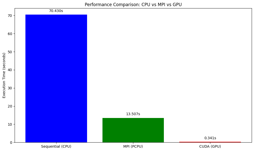
Performance Comparison Script
import matplotlib.pyplot as plt

# Extracted timings from the printed output
methods = ['Sequential (CPU)', 'MPI (PCPU)', 'CUDA (GPU)']
times = [70.430, 13.507, 0.341] # Replace the times with the times printed by running the above scripts

plt.figure(figsize=(10, 6))
bars = plt.bar(methods, times, color=['blue', 'green', 'red'])
plt.ylabel('Execution Time (seconds)')
plt.title('Performance Comparison: CPU vs MPI vs GPU')

# Add labels above bars
for bar, time in zip(bars, times):
    plt.text(bar.get_x() + bar.get_width() / 2, bar.get_height() + 1,
             f'{time:.3f}s', ha='center', va='bottom')

plt.tight_layout()
plt.savefig('performance_comparison.png', dpi=300, bbox_inches='tight')
plt.show()
Exercise: Resource Efficiency Analysis
Run the above python script to create a comparitive analysis between the different methods you used in this tutorial to understand the efficiency of different resources
Example Solution
This plot shows the execution time comparison between CPU, MPI, and GPU implementations.
Best Practices and Common Pitfalls
Resource Allocation Best Practices
- Match resources to workload requirements
- Don’t request more resources than you can use
- Consider memory requirements carefully
- Use appropriate partitions/queues
- Test with small jobs first
- Validate your scripts with shorter runs
- Check resource utilization before scaling up
- Monitor and optimize
- Use profiling tools to identify bottlenecks
- Adjust resource requests based on actual usage
Common Mistakes to Avoid
- Over-requesting resources
# Bad: Requesting 32 cores for sequential code #SBATCH --cpus-per-task=32 ./sequential_program # Good: Match core count to parallelization #SBATCH --cpus-per-task=1 ./sequential_program - Memory allocation errors
# Bad: Not specifying memory for memory-intensive jobs #SBATCH --partition=defaultq # Good: Specify adequate memory #SBATCH --partition=defaultq #SBATCH --mem=16G - GPU job inefficiencies
# Bad: Too many CPU cores for GPU job
#SBATCH --cpus-per-task=32
#SBATCH --gpus-per-node=1

# Good: Balanced CPU-GPU ratio
#SBATCH --cpus-per-task=4
#SBATCH --gpus-per-node=1
Summary
Resource optimization in HPC involves understanding your workload characteristics and matching them with appropriate resource allocations. Key takeaways:
- Profile your code to understand resource requirements
- Use sequential jobs for single-threaded applications
- Leverage parallel computing for scalable workloads
- Utilize GPUs for massively parallel computations
- Monitor performance and adjust allocations accordingly
- Avoid common pitfalls like over-requesting resources
Efficient resource utilization not only improves your job performance but also ensures fair access to shared HPC resources for all users.
Key Points
Different computational models (sequential, parallel, GPU) significantly impact runtime and efficiency.
Sequential CPU execution is simple but inefficient for large parameter spaces.
Parallel CPU (e.g., MPI or OpenMP) reduces runtime by distributing tasks but is limited by CPU core counts and communication overhead.
GPU computing can drastically accelerate tasks with massively parallel workloads like grid-based simulations.
Choosing the right computational model depends on the problem structure, resource availability, and cost-efficiency.
Effective Slurm job scripts should match the workload to the hardware: CPUs for serial/parallel, GPUs for highly parallelizable tasks.
Monitoring tools (like
nvidia-smi,seff,top) help validate whether the resource request matches the actual usage.Optimizing resource usage minimizes wait times in shared environments and improves overall throughput.
Wrap-up
Overview
Teaching: 15 min
Exercises: 0 minQuestions
Looking back at what was covered and how different pieces fit together
Where are some advanced topics and further reading available?
Objectives
Put the course in context with future learning.
Summary
Further Resources
Below are some additional resources to help you continue learning:
- A comprehensive HPC manual
- Carpentries HPC workshop
- Foundations of Astronomical Data Science Carpentries Workshop
- A previous InterPython workshop materials, covering collaborative usage of GitHub, Programming Paradigms, Software Architecture and many more
- CodeRefinery courses on FAIR (Findable, Accessible, Interoperable, and Reusable) software practices
- Python documentation
- GitHub Actions documentation
Key Points
Keypoint 1